(I wrote this review of “The Book of Why” by Judea Pearl and Dana Mackenzie for the Astral Codex Ten book review contest, but I was not selected as finalist… sigh.)

Prologue: Three Jews on the Internet

I had just finished my lunch at the college canteen. As I walked along the long tables to put away my tray, I joined the conversation of another small group of people. A fellow freshman—a guy with a prominent nose—was steaming with rage, his cheeks and forehead purple, his tone of voice confidently jolting like a sawtooth, because apparently some ignorant peasants, somewhere, believed it was possible to keep an artificial intelligence in a box.

I felt confused. Why was he so profoundly worried about this, uh, “problem”? So, I have a computer in a box… Uhm… Yes I have a lot of old computers in boxes, always stayed there, whatever. Maybe the cardboard will catch fire if the computer is kept on? No, wait, now I get what he’s talking about: the cooling system won’t work properly because air circulation is constrained in the box! He must be one of those who have a big custom machine with colored leds on the fans that leave a fancy afterimage and strange ports nobody ever uses and everything is overclocked and by shorting R435 with pin 99 and overfeeding (important) an additional bit gets written between each two other bits on the disk doubling the capacity.

Instead, he rage-explained to me that it was about a man named Mr. Yudkowsky whom people paid (?) so that he would convince them to press a fake button (??), under a confidentiality agreement (???).

I was even more confused, but this man was clearly on to something—he sounded so confident!—so I followed along. As we crossed the central bridge, he was wrath-expounding an experimental test of optimal agency:

The rules were SIMPLE, they would be given X dollars if they predicted the amount Y that the partner had predicted they would get given the expectation Z of a third party who would lose X – Y from an initial Q amount of dollars known to the first but not the second, and OF COURSE all they had to do was compute d/du P log(P), but these SIMPLETONS utterly FAILED because they would rather convince themselves that they really DIDN’T CARE about losing ten dollars because they were FREQUENTIST MORONS.

All the details in the quote above are wrong, because I was not getting anything of that. But I understood that there were these poor people who were handed a complicated puzzle I couldn’t even get in my skull in the first place, and by statal decree I was supposed to be good at math, and if every one of them got it right, they would probably gain 10 dollars, and of course they couldn’t really not want those 10 dollars so they were incredibly stupid to not be perfectly intelligent. For real? What contrived mind would conceive such a vexatious experiment? What’s wrong with this guy? Why am I even paying attention to what he says?

Five years later.

As I write these words, the frequentists are amassing at the gate. I don’t know how long we can resist. I’m reading translated foreign articles in the newspaper. I arrive at the general culture section, the one where I can be sure to find a “physicist” explaining that the “quantic” mysteries prove wrong the naive materialistic reductionists that pretend to determine what is true and false (as if!) when the possibilities of the mind are actually not bounded by such trivial preconceptions as logic, or a “philosopher” (quotes possibly redundant) highlighting how the weird syntax rules of the defunct language of three derelict guys in some remote country open up a new profound understanding of the universe that is forever forbidden to us due to our excessive reliance on technology which, let’s be honest, can’t really do anything for real, or an “intellectual” (quotes redundant) showing how teaching too much math makes people think in a rigid way such that they believe any religious bullshit that the current dictator wants them to believe.

The fool of the week is some “Pearl” guy who has discovered the secret of causality [sound of quivering flamelights]. Mankind went through an intellectual dark age where no one could discern cause from effect, but now, thanks to the genial heterodox work of Pearl, a causality revolution has sparked through the world. All paradoxes are solved. All doubts are cleared. By invoking the power of the do-operator, the most insurmountable of problems becomes a trivial exercise to the initiated. The article avoids ever mentioning what this do-operating consists of, it just states very clearly with a lot of words that you are supposed to do-operate stuff and you will gain final knowledge. I am so overwhelmed by the light of this revelation that I put away the newspaper, take a mental note to cancel my subscription (to avoid damaging my feeble mind with such a stream of profound truths), and never think about this again.

No! Wait! I’ve already seen this somewhere… Uh-uh-uh-uhm… Found, it was mentioned in that blog, Andrew Gelman’s blog. I like that guy! He’s friendly, once I used his gang’s statistical software because I couldn’t manage to do a complicated data fit for the weekly laboratory assignment, it took some time but it spat out the answer that I wanted to be true, so he’s a good guy. He also always gives useful advice, like how he always recommends being wary of implicit choices in your procedure that you will take to bend the result of the statistical analysis to give out precisely the answer you want, such as doing the fit in a different way until you think it works. Anyway, if this was featured on Gelman’s blog, it means it’s ok! It’s not something silly! It’s just the newspaper that—by chance—made Pearl’s work sound silly like the other silly (for real) stuff they usually write about.

After having determined as indisputable fact that Pearl was a reputable source of knowledge, “understanding anything by repeated application of a do-operator” sounded dignified and worth of investigation. In fact, it sounded much like “understanding anything by repeated application of Bayes’ theorem”, an advice originated from that weird man, Mr. Yudkowsky, that had been proven useful so many times. Indeed, I had been curious at times about what exactly that shady character had been pursuing with such knowledge; however, whenever I inquired about his writings, I was directed toward an incredibly long revised version of the Harry Potter novels, depicting a by magnitudes more wearisome protagonist than the original, and left it at that.

Now, Pearl appeared to have written various books on the topic, luckily in a very limited number of two. The titles were “Causality” and “The Book of Why.” After obtaining my pirated copies, I could see at once that the former was very long and full of “obvious proofs left to the reader,” while the latter was rather short and filled with funny drawings. My profound love of knowledge compelled me to opt for the most efficient means of acquiring new information, and thus I set forth on reading “The Book of Why.”

The book proved interesting in a lot of ways. It blended historical narration with a clear presentation of a mathematical theory of causation and many remarkable anecdotes. It would be a waste to spoil for the reader the pleasure of discovering herself all the gems of this work, so I will limit my recount to the three themes that most stuck in my mind.

Fisher is Evil

If you have ever read Jaynes’ book on Bayesian statistics, you may remember that R. A. Fisher, one of the fathers of what we now call orthodox statistics, often pops up as the villain of the situation. Jaynes is always dutifully respectful of Fisher’s accomplishments and technical competence, but I will venture to say that, between the lines, he is painting the figure of a shithead. He even underlines how Fisher had no sense of humor at all and would explode in rage at the minimum involuntary provocation, while his Bayesian counterpart—the distinguished Sir Harold Jeffreys [2]—was a very funny and nice old man who chatted amicably with his friends, making fun of Fisher. Also, he indicates that Fisher was an eugenist, although I could not sense if, in the view of the writer, that counted as an obvious negative due to its association with Nazi ideology, or if it was just meant as a statement of fact with no connotation.

Early in the book, Pearl too starts by pointing out Fisher’s bad character, in relation to the limited success of an early theory of causation by Wright, called “path analysis”, which in hindsight forms the basis of the one invented by Pearl decades later.

Although Crow did not mention it, Wright’s biographer William Provine points out another factor that may have affected the lack of support for path analysis. From the mid-1930s onward, Fisher considered Wright his enemy. I previously quoted Yule on how relations with Pearson became strained if you disagreed with him and impossible if you criticized him. Exactly the same thing could be said about Fisher. The latter carried out nasty feuds with anyone he disagreed with, including Pearson, Pearson’s son Egon, Jerzy Neyman (more will be said on these two in Chapter 8), and of course Wright.

And here’s from chapter 8:

In 1935, Neyman gave a lecture at the Royal Statistical Society titled “Statistical Problems in Agricultural Experimentation,” in which he called into question some of Fisher’s own methods and also, incidentally, discussed the idea of potential outcomes. After Neyman was done, Fisher stood up and told the society that “he had hoped that Dr. Neyman’s paper would be on a subject with which the author was fully acquainted.”

“[Neyman had] asserted that Fisher was wrong,” wrote Oscar Kempthorne years later about the incident. “This was an unforgivable offense—Fisher was never wrong and indeed the suggestion that he might be was treated by him as a deadly assault. Anyone who did not accept Fisher’s writing as the God-given truth was at best stupid and at worst evil.” Neyman and Pearson saw the extent of Fisher’s fury a few days later, when they went to the department in the evening and found Neyman’s wooden models, with which he had illustrated his lecture, strewn all over the floor. They concluded that only Fisher could have been responsible for the wreckage.

But most importantly, like Jaynes, Pearl dedicates an entire chapter to a topic where arguably Fisher plays the role of protagonist. It narrates the story of how it was discovered that smoking causes lung cancer. I have systematically been exposed to anti-smoking propaganda since childhood. At school they would periodically explain to us how bad smoke was using a lot of fancy diagrams of the human body. However, nobody ever bothered to quantify the seriousness of the danger. Consequently, I always presumed that it was a true but somewhat small statistical effect that was not trivial to see and as such it was important to convince people of its existence. Well, it turns out that, by modern standards, the effect had been farcically easy to notice the first time:

Before cigarettes, lung cancer had been so rare that a doctor might encounter it only once in a lifetime of practice. But between 1900 and 1950, the formerly rare disease quadrupled in frequency, and by 1960 it would become the most common form of cancer among men. Such a huge change in the incidence of a lethal disease begged for an explanation.

[…]

Of course Hill knew that an RCT was impossible in this case, but he had learned the advantages of comparing a treatment group to a control group. So he proposed to compare patients who had already been diagnosed with cancer to a control group of healthy volunteers. Each group’s members were interviewed on their past behaviors and medical histories. To avoid bias, the interviewers were not told who had cancer and who was a control.

The results of the study were shocking: out of 649 lung cancer patients interviewed, all but two had been smokers.

[…]

Doll and Hill realized that if there were hidden biases in the case-control studies, mere replication would not overcome them. Thus, in 1951 they began a prospective study, for which they sent out questionnaires to 60,000 British physicians about their smoking habits and followed them forward in time. (The American Cancer Society launched a similar and larger study around the same time.) Even in just five years, some dramatic differences emerged. Heavy smokers had a death rate from lung cancer twenty-four times that of nonsmokers. In the American Cancer Society study, the results were even grimmer: smokers died from lung cancer twenty-nine times more often than nonsmokers, and heavy smokers died ninety times more often. On the other hand, people who had smoked and then stopped reduced their risk by a factor of two.

What was the role of Fisher in this? He was the most famous statistician on Earth. He was a habitual smoker. And he thought that everyone else was dumb and he was always correct.

As the first results showing a connection between smoking and lung cancer appeared, Fisher stated that the correlation was due to an unknown hereditary factor that caused both smoke craving and increased lung cancer risk. His opinion was probably shaped by his quantitative studies of evolution and his eugenic views; he was used to attribute more importance to genes than other people thought they carried.

Due to previous historical developments (discussed elsewhere in the book) orthodox statisticians had never introduced a clear concept of causation, concentrating only on correlations. Thus, when Fisher insisted on his hypothesis, no one had a statistical tool ready to throw at the data to prove him wrong. Even when the data showed that the connection was so strong that it provably could not be only due to an unobserved confounder, he stuck stubbornly with his idea. The argument that sealed the presence of a causal connection goes as follows:

Cornfield took direct aim at Fisher’s constitutional hypothesis, and he did so on Fisher’s own turf: mathematics. Suppose, he argued, that there is a confounding factor, such as a smoking gene, that completely accounts for the cancer risk of smokers. If smokers have nine times the risk of developing lung cancer, the confounding factor needs to be at least nine times more common in smokers to explain the difference in risk. Think of what this means. If 11 percent of nonsmokers have the “smoking gene,” then 99 percent of the smokers would have to have it. And if even 12 percent of nonsmokers happen to have the cancer gene, then it becomes mathematically impossible for the cancer gene to account fully for the association between smoking and cancer. To biologists, this argument, called Cornfield’s inequality, reduced Fisher’s constitutional hypothesis to smoking ruins. It is inconceivable that a genetic variation could be so tightly linked to something as complex and unpredictable as a person’s choice to smoke.

This was not at all clear to me on first reading, so I made a diagram:

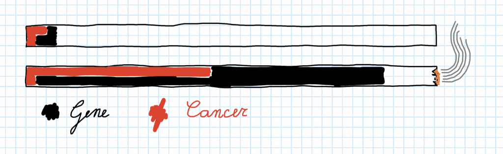
The two bars represent non-smokers and smokers. I arbitrarily filled two ticks of the non-smokers with cancer (red), and two ticks with the cancer-smoke-gene (black), with one tick of non-smokers having both cancer and the gene.

Since smokers have nine times the risk of getting cancer, I have to fill 2 x 9 = 18 ticks with red in the smokers bar. How many ticks should be filled with black? First, if it’s only the gene which is causing the increase in cancer risk, all additional red ticks compared to the non-smokers must also be filled with black, so I filled with black the 16 ticks from 3rd to 18th. Second, within the people who have the gene, the fraction of cancer must stay the same: otherwise being a smoker would have an additional effect on cancer not explained by the gene. In the non-smokers bar there is one red tick out of two black ones, a proportion of 1:2, while in the smokers bar there are already 17 red-black ticks, so I have to add another 17 black-only ticks.

This shows that the fraction of smokers who have the gene must be at least nine times the fraction of non-smokers who have it, which is the first part of the reasoning. Then it follows that the fraction of non-smokers with the gene is less than 1/9, otherwise more than 100 % of the smokers would have it. The argument concludes by stating that of course it is very unlikely that just 1/9 = 11 % of the non-smokers have the gene, there must be more, and so the premise (only the gene is having an effect on cancer) is false.

I’m no biologist, so I did not understand why there could not be less than 11 % non-smokers with the gene. I asked a biology student, he said “Muh I don’t know.” I asked a statistics student, she said “Uh well you just get used to a certain magnitude of genetic effects after seeing many of them and this seems too strong.” To this I objected: but there exists also genetic (or innate anyway) stuff that has a strong effect on everything, right? For example, if you are born with an additional X chromosome, you are more at risk of doing all sorts of weird stuff like throwing away clothes because they have holes, hanging up little icons of Jesus, spreading dangerous chemicals on domestic surfaces, etc. Or if you are born intelligent, you will fare better than other people at school without breaking a sweat and also have fun while doing it and get a higher salary without moral compromises and physical labor. In fact, X-X humans do smoke less and live longer and are better at school than X-Ys. The same goes for intelligent people. So how can an innate factor be excluded here?

I think the explanation is “implicit deconfounding.” Gender does have a strong effect on death and smoking. However, it is not a problematic confounder, because it is very easy to know the gender of people [citation needed]. So, even if you don’t mention it, of course if the gender effect was relevant to the matter at hand you would have noticed and adjusted for it. Remember that the final goal of this kind of discussion is prediction: if medical science was so advanced that you could tell beforehand if you are the kind of guy who would stay healthy even in the face of smoking, nobody would care about the average causal effect of smoke on cancer in the population, the thing would stop being statistical (well, let’s say “become less statistical”) and you would ask your doctor if you in particular can smoke or not because, doctor, I really like getting high on marginal cancer risk.

This applies to genetic/innate factors in general in the following way: it is true that we have examples of very strong and influential factors, and not just weak ones. But strong factors tend to have an effect on everything, not just a single habit and a single medical outcome, in such a way that you already know of those factors beforehand and they never qualify as confounders. It is interesting that indeed there is a genetic effect matching Fisher’s hypothesis:

Ironically, genomics researchers discovered in 2008 that Fisher was right: there is a “smoking gene” that operates exactly in the way he suggested.

However:

The discovery of the smoking gene should not change anybody’s mind about the overwhelmingly more important causal factor in lung cancer, which is smoking. We know that smoking is associated with more than a tenfold increase in the risk of contracting lung cancer. By comparison, even a double dose of the smoking gene less than doubles your risk. This is serious business, no doubt, but it does not compare to the danger you face (for no good reason) if you are a regular smoker.

So in hindsight it was reasonable to expect the presence of an innate common cause, but it was also reasonable to expect that it could not be big enough to explain all the observed effect without having been noticed already.

Far atop these paragraphs it is clickbaited: Fisher is evil. Let us flesh this out in more exquisite detail. Pearl and Mackenzie say:

The case of Fisher is particularly sad. Of course, skepticism has its place. Statisticians are paid to be skeptics; they are the conscience of science. But there is a difference between reasonable and unreasonable skepticism. Fisher crossed that line and then some. Always unable to admit his own mistakes, and surely influenced by his lifetime pipe-smoking habit, he could not acknowledge that the tide of evidence had turned against him. His arguments became desperate. He seized on one counterintuitive result in Doll and Hill’s first paper—the finding (which barely reached the level of statistical significance) that lung cancer patients described themselves as inhalers less often than the controls—and would not let it go. None of the subsequent studies found any such effect. Although Fisher knew as well as anybody that “statistically significant” results sometimes fail to be replicated, he resorted to mockery. He argued that their study had showed that inhaling cigarette smoke might be beneficial and called for further research on this “extremely important point.” Perhaps the only positive thing we can say about Fisher’s role in the debate is that it is very unlikely that tobacco money corrupted him in any way. His own obstinacy was sufficient.

(Note: the part on “tobacco money” does not mean he was not paid by big tobacco, it means he was paid but only because he was already a supporter and would have been in any case.)

So, well, I don’t think Fisher is “evil” as, like, the idealized evil dictator of eviland. It’s his unfortunate circumstance that’s evil! Fisher is not evil, he is, let’s say, the rationalist nightmare. He’s a sort of genius, brilliant at math, always the smart guy in the room. From his point of view all the dumbwits around him are making mistakes at each turn so he invents a new statistical language which limits by construction answerable questions to objective ones and constrains other people to only use methods designed and vetted by a caste of trained statisticians led by him such that nobody can ever make mistakes or try to ask subjective questions, problem solved.

(Spoiler: it ends with people just being confused and misusing the language to prove any bullshit, folks there are no true Scotsmans here to see, it’s just unfounded rumors, please return to your homes.)

Then, from the evident fact that everyone else is dumber than him, he’s ready to see that innate intelligence and ability are extremely important factors, he sets out to do something concrete about this and studies how to systematically improve the intelligence of people for the benefit of mankind (eugenics).

(Spoiler: it ends with people applying eugenics as “So I’ve measured that the elliptical eccentricity of the craniums of this group of Africans is 0.02 less than that observed on my friends, which necessarily implies negroes are designed by God to be slaves, so let’s kill all Jews!”)

Then a new group of dumbsters pops up saying that his favorite drug, which has clearly no side effects and helps him concentrate, which surely is a benefit to humankind since this enables his intellect to run at top speed and produce more scientific breakthroughs, causes cancer. WTF causality is an illusion simpletons, even babies know that nowadays, and of course you want a scapegoat for your inferior genes. Now tell me, a literal additional chromosome can cause you to have a literally bloody hole between your legs or to be literally diagnosed with dumbness, and now oh yes these people we have found who can’t avoid drugs and have cancer can’t be a genetic effect woooo man it’s tooooo complicated to be a genetic effect.

(Spoiler: it ends with people thinking that maybe inhaling burned stuff is not so bad and it gets soft-banned very slowly causing—yes, causing indeed—millions of additional easily preventable deaths.)

So, now I ask you: what would you have done in Fisher’s shoes? Like, Fisher almost nailed everything, just, in a sort of everything goes wrong in practice way. What thought process could have brought you away from a mental state in which all the pieces of reality feel so connected?

Maybe you could have solved it with expected utility: from your point of view you feel quite sure about the genetic explanation, but if it turns out smoking is bad, and in the meantime we have not stopped it, the outcome is a pile of bodies! So we stop smoking while we figure out the situation, we can always light back our pipes later. But this works poorly in practice due to Pascal’s milking: what if the loss of quality of life of people who like smoking balances the additional deaths? What if Fisher can’t concentrate and find a breakthrough that brings to important discoveries in all fields through a new statistical analysis method? What if God exists and thinks YOU SHALL SMOKE? What if racism is so bad that any second you dedicate to stopping smoke is wasted and should have been dedicated to fighting racism instead so you should stop thinking about this right now? What if Pascal comes back from the dead because zombies and eats your face? How can you smoke without a face?

Yes I’m a whig historian so what?? Pearl is, too.

[Edit June 8, 2022: Gelman posted about this topic, there’s some discussion in the comments]

The Monty Hall Paradox

Why is the Monty Hall problem so counterintuitive?

I assume that most readers are familiar with this paradox, but, in case you don’t know about it, here it is:

In a TV game, there is a prize (a car) hidden behind one of three closed doors. The other two doors contain goats because our decadent western culture doesn’t value goats any more. You try your luck and pick one door. Before opening your door, the host opens another door, revealing a goat! Then he asks you if you want to go on with your choice or switch to the remaining door. What do you do? Think about it then look up the solution on the Wikipedia article.

Done? Now I’ll tell you about the first time I encountered this thing. I was at a Physics summer camp. At dinner, one guy is running the show by flabbergasting us with all sorts of counterintuitive trivia. Like, did you know that whenever you copy a file the computer introduces thousands of errors in the copy? Then he starts telling about this survival puzzle where you have two doors and there is a tiger behind one of them. He asks: what door do you choose?

Me: …

No ok wait there are three doors, and one leads to the tiger. And one leads to the goat. No wait wait I have it there are two goats, one tiger, you are about to open the first door, but your dumb comrade that never agrees opens the second door and finds a goat. The weird fact is that now you should switch to the third door if you want to find the tiger!

Weren’t we trying to avoid the tiger?

Ahahah I’m dead then—uhm—yes well it’s the same it means you have to go on with the first door, but now you are more sure it does not contain a tiger. And this just by opening an unrelated door with a goat.

I don’t believe this. Our choices are not related in any way to the true tigerness of the doors, so it should make no difference if, excluded the second door, I switch between the first and third.

I know, I know, it’s paradoxical, but it works for real! Because: the total amount of tigerness in the first door is still 1/3 from before, but the tigerness in the third door is 1/2 now, so the first is safer.

I’m still not convinced. This is about probabilities, so imagine repeating the situation many and many times over, each time assigning the tiger to a door at random. Excluded the unlucky to order 0 cases in which the dumb friend meets death immediately, by symmetry the times where the tiger was in the first door are as many as those where it was in the third, because we can relabel the doors switching 3 and 1 without this affecting the randomness of the assignment.

Mmmmm I’m not sure, you want to avoid the tiger in your once-in-a-lifetime specific situation, it does not make sense to think about what you would do in a hypothetical repetition. I think you should compute probabilities in the way I showed you, directly with what you know at each step of the game.

No, because by the law of large numbers, the probability is the relative number of times something happens if you imagine repeating it infinite times. So if the result is different, there must be something wrong in your reasoning.

Ok… if you invoke the law of large numbers, I think it’s powerful enough to dispel the paradox.

Whiz reader quiz: was the avoid tiger version equivalent to the original achieve car version? Spoiler: not at all, the trick doesn’t work any more! Think about it then read the Wikipedia article, without skimming this time!

[Dear anonymous dinner time storyteller: I’m doing an injustice to you. An injustice because probably you told the paradox in the correct way for it to be a paradox instead of the wrong way I’m retelling it such that I happen to be right. Moreover, I never made such well rounded arguments involving symmetries and probabilities, I just shouted “BUT LAW OF LARGE NUMBERS!!!” But, you see, now I have piled academic credentials over academic credentials, my path is strewn with the dead bodies of squirrels, and I can write my version of the story on a popular blog for everyone to read and laugh about your stupidity. WHO CONTROLS THE TIGER NOW?]

Now that the filler story intended to stop the reader from easy-peeking the solution is over, we can resume with what Pearl has to say about the paradox. The most important thing is:

Paul Erdos, one of the most brilliant mathematicians of modern times, likewise could not believe the solution until a computer simulation showed him that switching is advantageous.

This is extremely important because not getting Monty Hall’s paradox kept a dent in my pride for a long time and now, thanks to Pearl, I can say “not only PAUL ERDOS himself got it wrong, he wanted to see EXACTLY THE SAME THING I wanted, an infinite repetition of the experiment.” (Yes, I know, it was already in the Wikipedia article, but I wasn’t reading the English Wikipedia article at the time, you anglo-entitled colonizers!)

Now that my honor is reestablished, we can look at minor details, like understanding the paradox.

Pearl argues that the paradoxical quality of this problem stems from the instinctive tendency of humans to search for causal explanations. “My arbitrary choice of door cannot cause the car to switch door!” Yet the probability changes, without involving any causation. It’s just probabilities, and your brain isn’t wired to weigh plausibility under uncertainty, it’s wired to blame people, which involves finding the cause of something such that you can put blame on it. There are other important details that matter, like in the tiger example above where it’s indifferent to switch door due to a slight modification of the problem, but the reason why the result appears strongly counterintuitive to many people, even when given unambiguously the correct statement, must reside in how we innately tend to represent the situation in our mind.

I could go on Pearlsplaining all this stuff with causal diagrams, like I planned many years ago. But then I thought: who cares? I mean, people who really care will read Pearl’s book anyway. Probably the serious one instead of the dummy version I’m reading because I’m lazy. So, how do I actually explain this stuff in a way that appeals to people who would probably never spoil their free time reading a math textbook?

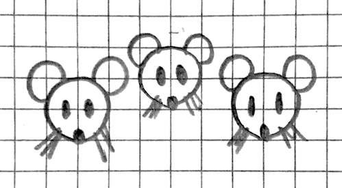
I was wondering about this while walking in the woods at sunset, and as usual I started a mental dialogue with an imaginary interlocutor. So this interlocutor wanted to know what was I talking about, and I started explaining all things about arrows of causation, confounders, etc. As I explained he interrupted continuously asking all sorts of mischievous mathematical questions aimed at finding a crack in any step of my reasoning, so at some point I realized I was imagining a synthesized version of my university friends or maybe myself. But, who would want to discuss with a persnickety fake Physicist? So I switched to imagining a nice girl, a mythical creature appearing in the narrations of those brave people who ventured outside of the Physics department and managed to come back, who in the stories always listens to everything you want to say, and then in the end always pats you on the head and says you are a “good little mouse.”

The imaginary girl—the image of whom was just a faint ghost in my mind because nobody can see its true appearance and survive, they say—dutifully listened to my ramblings, without ever interrupting. But this turned out to be a double edged sword, because at some point I could sense I was losing her! She was getting bored! What a new, difficult kind of daunting task I had set myself up to… I had to keep entertained an idealized girl! How to accomplish this? I ran the squirrels hard and got some ideas about it; putting in some effort, finally I managed to produce a dialogue with a girl explaining Pearl’s version of the Monty Hall paradox without losing her attention.

You are about to read this dialogue. There is, however, a slight difference with respect to the original version. Some friends read an early draft and advised me to revise it because it sounded too “misogynist.” It is a Greek word which means “against females.” So I asked what has this to do with females, and they started to say confused stuff about like it’s not really against, but it might sound like you assume that the girl is not getting this and that, you see, because depending on the context, etc. The little lecture sounded like they were going around something without quite getting at it. I couldn’t see clearly, but after a while, I don’t know how, I started to parse the babble. Connect the dots. And all of sudden, a revelation struck me with full force, strong and pure in its simplicity, putting all the pieces of the puzzle together at once: the females were the girls all along!

So I changed the interlocutor from “girl” to “female” to remove the unintended misogyny.

Me: Do you know about the Monty Hall Paradox?

Female: Yes.

Me: Wrong answer, I’ll explain it to you. There’s a TV game show with three doors of which you have to pick one. Behind one door there’s a car, behind the others there are goats. It is assumed that you want to win a car and not a goat. The host (Monty Hall) lets you choose a door, let’s say you choose door number 1. But before opening it, to waste time, he opens door 2 and finds a goat (of course he already knew that it didn’t contain the car, otherwise he would spoil the game). Then he asks: “Now that you have seen a goat behind door 2, do you still want door 1 or switch and choose 3?” What should you do? Switch, stay, or it doesn’t make a difference?

Female: Wouldn’t these goats bleat? Anyway I told you I already know, you have to go with 3.

Me: Ok, but why should you choose 3?

Female: List all possible cases, count those where you win if you pick 3, there’s more, done.

Me: Ok, but it’s a paradox because it shouldn’t be the intuitive answer, isn’t it? The intuitive answer is that it makes no difference; once you have excluded door 2, the fact of having chosen door 1 beforehand doesn’t make it more or less likely that door 3. And the goat is a silent animal.

Female: So, these penises you promised earlier?

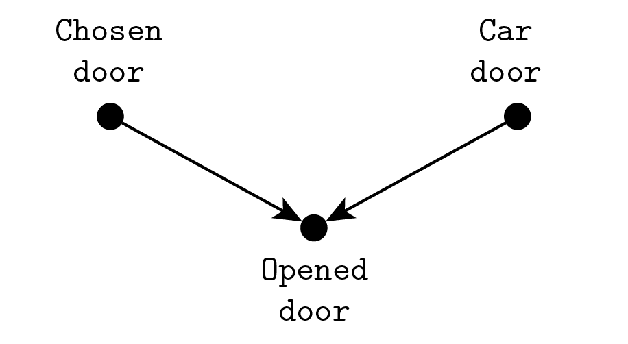
Me: In a moment, we first have to draw a causal diagram. Consider these three variables: which door hides the prize, which door you have chosen, which door Monty Hall opens. Imagine representing them with little dots and linking them with arrows, where each arrow goes from cause to effect. So we have to link the prize door to Monty Hall’s one, because he can’t open the prize door, and also the chosen door because he can’t open that either.

Female: Good, he’s drawing arrows now. [makes a well-known gesture with the hands]

Me: The point of this diagram is that in general when you have two causes of the same variable, and you know what value the variable yields, a correlation pops up between the two causes, even if there isn’t a direct causality relationship between them.

Female: So wouldn’t the arrows run opposite? Like, the way you say it, the effect has an effect on the cause, it doesn’t make sense.

Me: It’s an epistemological thing, what you know about the effect has an effect on what you know about the cause. For example, if you find a bite, you infer you have been bitten by a mosquito, but the cause of the bite is the mosquito.

Female: So you managed to make the obvious clear as mud. Epistonks. About that, the dicks?

Me: Imagine that I take you and your mother

Female: Oh!

Me: …and send you around with a little notebook to stop people at random and measure their penis length. When you measure them they are erected, when your mother does, they are not.

Female: This really must have set your brain back some juice. But wouldn’t my mother get some erections too? Didn’t you like mature women?

Me: It doesn’t matter, it’s a statistical thing, it is actually sufficient that you get harder mickeys than mom on average. On your adorable little notebooks you pencil down age and length. Finally you bring the notes back to me, I fill an excel and group the data by penis length rounded to the centimeter.

Female: And find out that you got a small one.

Me: No, in each group I compute the mean age separately for yours and mom’s, and it turns out that—surprise!—for any penis length, yours are younger.

Female: Surprising as fuck! Should I stop oldtimers??

Me: But I told you to stop people at random! At random means like drawing from an urn, you can’t pick them!

Female: Man you made your example yourself!

Me: But… Listen, the point is: from this analysis, could I infer that you girls contravened my crystal clear scientific directions? Nope, because it’s actually a paradox equivalent to Monty Hall. The finding that you measured younger guys is a statistical illusion, much like the correlation between the door you fix on initially and the one with the prize. Ok actually the anticorrelation because you have to switch door.

Female: But: if I really have to change the door, then it is not an illusion.

Me: Whatever, it’s an illusion in the penises case, what the two examples share is an unexpected correlation. Anyway, it becomes evident if we draw the diagram:

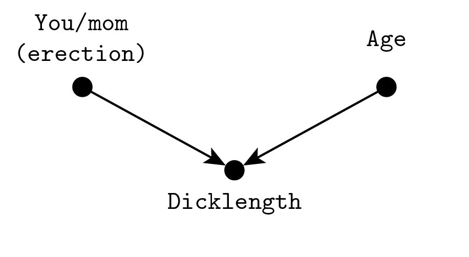
Me: So, who out of you and your mother is carrying out the measurement influences the length due to the differential erection rate. Age matters too because children have it small.

Female: Every mile a pedo-phile, du-di-du….

Me: …The arrow structure is the same as before, and the other thing in common is that the variable influenced by the other two is the one we are “fixing”: with doors, we know which door Monty’s opened, with penises, I group by length and do the calculation one length at a time, so it’s like it’s fixed.

Female: A nice story. Let me guess: the moral is that I shouldn’t judge males based on their equipment.

Me: Yes but do you get why this happens? If you take some guys who all have dicks of equal length, you will have some kids and some adults. But to have a little kid with a penis as long as an adult, you need the kid to be on a boner but not the adult, and so this correlation comes about.

Female: Ok. You gifted me your pearl of scientific wisdom. Yet, following this line of reasoning, I still don’t see why should I change door.

Me: Well, so. Both erection and age have a positive effect on dicklength, more erection more age more dick, and the result is an anticorrelation. Conversely, the initial door taken and the winning door both have a negative effect on the suregoat door, because Monty must avoid them both. So, in the second case too, we have an anticorrelation (between first choice and prize), because two minus signs make a plus. If you are confused by this thing about signs, think from the start using “negerection” and “negage.”

Female: Aha.

I hope to have debored you enough and that from now on you will remember what these vagina diagrams are about. Their actual boring name is “causal colliders,” by the way, because of the arrows “colliding” in the central variable.

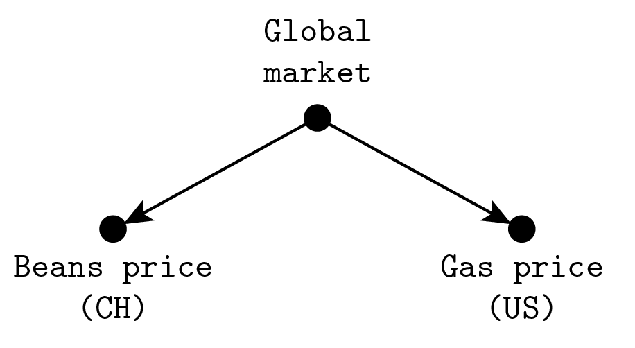
But this is only the beginning! Because Pearl’s point is more subtle: the paradoxiness  depends on the direction of the arrows. “Spurious” correlations happen all the time without you getting confused about what’s the true relationship of cause and effect. Probably you have already heard common examples like “correlation is not causation, because if you find out that the price of beans in China is correlated with the price of fuel at the station, it doesn’t mean that a shopkeeper in Beijing can make you pay more for a tankful by raising his prices, it’s the global market trend which is the common cause that makes them correlated.” However, for completeness’ sake, I will provide yet another example just for my dear reader.

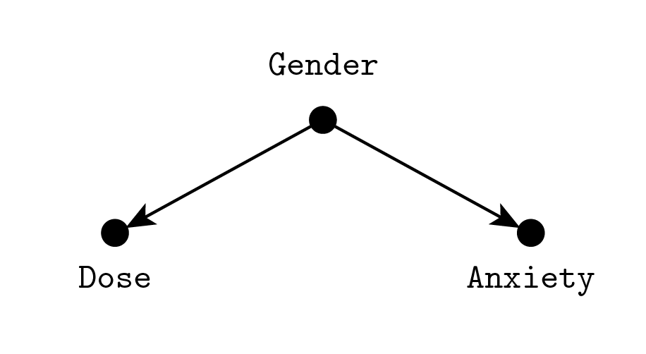
Suppose that the Distinguished Quacky B. Quackson High Quack Chair Professor of Applied Quacking at McQuack University is running a study to prove that their new Quackopatic treatment for anxiety works. Also, suppose he is at odds with Fisher (easy call) so he won’t use Fisher’s randomized controlled trial (RCT) technique with a control group. He designs the study in the following way: he takes in people with self-declared anxiety problems. Since a lot more women answer the call, he stratifies the sampling by imposing the same number of men and women, to do a balanced study on both sexes. He doses the drug proportionally to body weight. A week after treatment, he has subjects fill a questionnaire on anxious behaviors and—success! There is a very strong negative correlation between self-reported anxiety and the amount of medicine administered. You know the full story because I’m kind, he just reports the result as “we observed a very strong negative correlation between medication and target, pointing without doubt to the effect of the treatment” omitting all the other fussy details. Now tell me: why shouldn’t you place too much trust in Prof. Quackson’s words? Do you see a reason why the correlation is not meaningful?

…

…

…

Don’t look at the solution yet! Think!

…

…

…

And don’t you dare find one of those other zillion reasons for not trusting Prof. Quackson’s study which have nothing to do with the point!

…

…

…

Done? The solution is: the sample of women is more anxious than the sample of men. And he is giving more Quacksulveforax (that was the name) to male subjects because they weigh more. So the correlation is just the prior sex-anxiety correlation, he would observe it even before the treatment.

I expect that you either have figured out the solution yourself, or at least think that the solution makes sense. Actually, I hope that you are already thinking about how to fix the study. It would be sufficient, say, to compute the correlation separately for males and females. Or to measure the difference in anxiety pre- and post-treatment. Or have a control group. I expect that how you feel about this stuff is of course it doesn’t work! Just do the study in the right way!

While, instead, I expect you to feel perplexed about switching door or trusting your assistant not to have cherry-picked young subjects for the penis experiment. What’s the difference in trying to see through the veil of the correlation between these two kinds of situations? Pearl’s answer (to everything, actually) is: just draw the graph!

The arrows go in the opposite direction! It is easy for us to understand the correlation when it is produced by a shared cause of multiple effects, while it is difficult to have an intuitive grasp when there’s a single effect of multiple causes.

I don’t feel sure about this explanation, because there are cases where we are very quick at reasoning in the correct way even with colliders. Someone depleted the secret stash of chocolate. Was it little Anny or little Benny or little Chenny or…? If you find sure proof that Anny ate the chocolate, how much time do you lose trying to check if also Benny, Chenny, Danny, etc. took part in the misdeed?

The Ladder of Causation

Pearl was once all for a purely probabilistic model of causality. Then one day he was climbing the ladder to his mezzanine henhouse (Jews have to raise their own hens because Jews), one hook broke and he fell down banging his head badly on the floor. It was reported that, during the trip to the hospital, he grumbled continuously half-unconscious “THE LADDER, THE LADDAHER…” He was kept in intensive care for one week. On the morning of the seventh day, he woke up and stood. The nurse got mad, put him back down on the bed and called the doctors. All the doctors came around him, who was still on the bed but had raised his back and was sitting against the headboard. He looked at them wearing his typical sly smile. The doctors asked how he felt, and thus he spoke: “THE LADDER IS THE CAUSE. THE CAUSE IS THE LADDER. ONLY AT THE TOP OF THE LADDER THE EFFECT SUCCEEDS THE CAUSE. THE CAUSE IS AT THE TOP OF THE LADDER. THE LADDER IS A LADDER OF CAUSATION.”

Mr. Pearl, how do you do? Can you look at my hand?

I SHALL LOOK.

Good. Now tell me, given that the ratio of patients hospitalized for head injury to the other patients is 1:200, and that the probability of failing the medical finger count test after a head trauma is 10 times the one in normal conditions, and that I’m showing you two fingers, what is the probability that you banged your head?

Pearl was still smiling. He clenched the doctor’s hand and broke all his fingers.

Seriously version

Seriously, you still wasting time, Rubin? Can you get your act together at last, please? Do you think that the Nobel to Imbens saves your sorry mustache? You would just need for once to compute, step by step, the probability that the identity of your father is correct, and you would immediately recognize the usefulness of causal diagrams. The light would shine through the equations.

Serious version

Pearl begins his book with the Genesis:

I was probably six or seven years old when I first read the story of Adam and Eve in the Garden of Eden. My classmates and I were not at all surprised by God’s capricious demands, forbidding them to eat from the Tree of Knowledge. Deities have their reasons, we thought. What we were more intrigued by was the idea that as soon as they ate from the Tree of Knowledge, Adam and Eve became conscious, like us, of their nakedness.

Of course the Old Testament, as a good and proper sacred text, already embodies all truths, and in particular proves Pearl right on his theories. (Is Jesus a redundant set of parameters? Or is Jesus an even more compact representation of the Truth?) Anyway, after a biblical tour, Pearl lands us on the Ladder of Causation. The Ladder has three rungs, which correspond to increasing abilities of an intelligent agent in the manipulation of causality.

Rung one is the ability to see, to observe relations and associations between things. Probabilistic reasoning belongs here: I notice that of all the times $A$ happens, in a fraction $p$ of those, $B$ follows $A$. Then I say that $p$ is the probability of $B$ conditional on $A$, $P(B|A) = p$, and, if I see $A$ again, I predict that $B$ will happen with probability $p$. Every Monday, school finishes one hour earlier than usual, and you have to go home on foot. Sometimes, as soon as your house is in sight, you see a group of men rushing out from the backyard. Thus you estimate $$\begin{align}A &\equiv \text{get home early,} \\ B & \equiv \text{see weird men,} \\ P(B|A) &= \begin{cases} \frac1{5\times\text{Nr. Mondays} + 2} & \text{if $A$ is false,} \\ \frac{\text{Nr. times saw men} + 1}{\text{Nr. Mondays} + 2} & \text{if $A$ is true.}\end{cases}\end{align}$$ Rung two is the ability to do. Instead of waiting for $A$ to happen naturally, you force it to be true somehow, and compute again the probability of $B$ given having done $A$, $P(B|\hat A)$, where $\hat A$ (A with a hat) is a shorthand for the proposition “$A$ is true, but not by the usual mechanism left implicit in the initial definition of $A$, but by some other mechanism I employ to make it surely true in a specific case.” An equivalent notation is $P(B|do(A))$, which earns it the fancy name “do-operator.” Depending on what was the original process that brought about $A$, this probability may be different from $P(B|A)$. To investigate the provenance of the odd evasive folks, you decide to come back one hour earlier on Tuesday. Intuitively, this will tell you if the point is the weekday (Monday) or coming back before time. The point being that the point is the cause. You give an excuse to the principal and head home. This time you don’t notice any strangers escaping, but your mother seems very worried about your anticipated exit.

«My little mouse, how can you be home so early? It is not Monday, isn’t it?»

«Mmm nothing mom, I just… I got a very strong headache, I think I played too many video games yesterday night, and the teacher was kind and let me go home earlier.»

«Oh dear! But the school must call me before they let you out! They are mandated to confirm permission with the parents!»

«Listen mom don’t make a case of it, anyway I already feel better, don’t worry, I took two aspirins»

«Yes yes but how dare they send you out earlier in this way without informing me beforehand! This is utterly unacceptable! I must request a personal colloquy with every teacher!»

«Please mom no, it’s embarrassing, mmmalso I gave an excuse to the teacher, don’t tell them I was at the console until 3 am, teachers are so finicky about this stuff…»

“But I can’t let this thing pass! It is against the rules! I’m completely positive that this is against all the rules!»

«Mom I know you are anxious but the’re no dangers around here, ok? Like, I do it every Monday, it doesn’t change if you don’t know that I’m out, I’m fine»

«I can see very well that you are fine! But you can’t get home early without telling me first!»

Rung three is the ability to imagine. You know that $A$ happened, followed by $B$. But… would $B$ have happened if $A$ had not? Notice this is not the probability of $B$ given not-$A$, $P(B|\neg A)$, neither the probability of $B$ given making $A$ not happen, $P(B|do(\neg A))$. You already know that, in the case at hand, $A$ is true and $B$ too, and you didn’t lift a finger to call for $A$. The fact that they turned out to be true could change your assessment of what would have happened in that specific circumstance if $A$ was forced to be false. So you need to imagine not just something you don’t know, but something which contradicts your factual knowledge. This kind of thinking is called counterfactual. Your mother is again a deep source of examples, left as exercise to the reader.

Mother-free and any gender-relatable concept-free this time I promise version

So, the ladder of causation… without mothers? Whatever. Well, the ladder is not just a way to hang three concepts on a wall to satisfy the rule of three, it implies a hierarchy. (A rungarchy?) To move up one rung in the ladder, you need new mental tools and concepts that weren’t required to find your way around in the lower rung. Pearl relates this to the level of general intelligence:

So far I may have given the impression that the ability to organize our knowledge of the world into causes and effects was monolithic and acquired all at once. In fact, my research on machine learning has taught me that a causal learner must master at least three distinct levels of cognitive ability: seeing, doing, and imagining.

The first, seeing or observing, entails detection of regularities in our environment and is shared by many animals as well as early humans before the Cognitive Revolution. The second, doing, entails predicting the effect(s) of deliberate alterations of the environment and choosing among these alterations to produce a desired outcome. Only a small handful of species have demonstrated elements of this skill. Use of tools, provided it is intentional and not just accidental or copied from ancestors, could be taken as a sign of reaching this second level. Yet even tool users do not necessarily possess a “theory” of their tool that tells them why it works and what to do when it doesn’t. For that, you need to have achieved a level of understanding that permits imagining. It was primarily this third level that prepared us for further revolutions in agriculture and science and led to a sudden and drastic change in our species’ impact on the planet.

I cannot prove this, but I can prove mathematically that the three levels differ fundamentally, each unleashing capabilities that the ones below it do not.

The emphasis is mine. Elaborating further on this, Pearl explains he sees current statistics/machine learning research as stuck on rung one:

The successes of deep learning have been truly remarkable and have caught many of us by surprise. Nevertheless, deep learning has succeeded primarily by showing that certain questions or tasks we thought were difficult are in fact not [come on man!]. It has not addressed the truly difficult questions that continue to prevent us from achieving humanlike AI. As a result the public believes that “strong AI,” machines that think like humans, is just around the corner or maybe even here already. In reality, nothing could be farther from the truth. I fully agree with Gary Marcus, a neuroscientist at New York University, who recently wrote in the New York Times that the field of artificial intelligence is “bursting with microdiscoveries”—the sort of things that make good press releases—but machines are still disappointingly far from humanlike cognition. My colleague in computer science at the University of California, Los Angeles, Adnan Darwiche, has titled a position paper “Human-Level Intelligence or Animal-Like Abilities?” which I think frames the question in just the right way. The goal of strong AI is to produce machines with humanlike intelligence, able to converse with and guide humans. Deep learning has instead given us machines with truly impressive abilities but no intelligence. The difference is profound and lies in the absence of a model of reality.

Just as they did thirty years ago, machine learning programs (including those with deep neural networks) operate almost entirely in an associational mode. They are driven by a stream of observations to which they attempt to fit a function, in much the same way that a statistician tries to fit a line to a collection of points. Deep neural networks have added many more layers to the complexity of the fitted function, but raw data still drives the fitting process. They continue to improve in accuracy as more data are fitted, but they do not benefit from the “super-evolutionary speedup.” If, for example, the programmers of a driverless car want it to react differently to new situations, they have to add those new reactions explicitly. The machine will not figure out for itself that a pedestrian with a bottle of whiskey in hand is likely to respond differently to a honking horn. This lack of flexibility and adaptability is inevitable in any system that works at the first level of the Ladder of Causation.

So, Pearl has a three-bullet model of reality that explains evolution and the secret to artificial general intelligence? I think I’m starting to hear the knocks of a hammer… Ah wait that’s Ukraine’s invasion. But then tell me, when was the last time that a baby Jew geezer changed our foundational understanding of the world with a few simple equations? Ah it happens every time you say? Cool, I’ll try to be more sympathetic then. Maybe Pearl, when he says that he has proven mathematically that the three levels differ fundamentally, is just trying to churn out a convincing prose. What’s his say on this?

Decades’ worth of experience with these kinds of questions has convinced me that, in both a cognitive and a philosophical sense, the idea of causes and effects is much more fundamental than the idea of probability.

[…]

The recognition that causation is not reducible to probabilities has been very hard-won, both for me personally and for philosophers and scientists in general.

[…]

However, in their effort to mathematize the concept of causation—itself a laudable idea—philosophers were too quick to commit to the only uncertainty-handling language they knew, the language of probability. They have for the most part gotten over this blunder in the past decade or so, but unfortunately similar ideas are being pursued in econometrics even now, under names like “Granger causality” and “vector autocorrelation.”

Now I have a confession to make: I made the same mistake. I did not always put causality first and probability second. Quite the opposite! When I started working in artificial intelligence, in the early 1980s, I thought that uncertainty was the most important thing missing from AI. Moreover, I insisted that uncertainty be represented by probabilities.

[…]

Bayesian networks inhabit a world where all questions are reducible to probabilities, or (in the terminology of this chapter) degrees of association between variables; they could not ascend to the second or third rungs of the Ladder of Causation. Fortunately, they required only two slight twists to climb to the top. First, in 1991, the graph-surgery idea empowered them to handle both observations and interventions. Another twist, in 1994, brought them to the third level and made them capable of handling counterfactuals. But these developments deserve a fuller discussion in a later chapter. The main point is this: while probabilities encode our beliefs about a static world, causality tells us whether and how probabilities change when the world changes, be it by intervention or by act of imagination.

The list goes on. So it wasn’t just a single episode, Pearl has set up an electoral campaign team, a troll factory and a go-go-Pearl! anime pin up ballet to convince you that you can’t just climb the ladder of causation with your probability calculus when you fancy it, learn your place and stay on the lower rung, only the initiates can ascend the sacred ladder.

Wait, wait, wait, wait. I understand that spiritual fanboys will get their mystic orgasm out of all this and feel compelled to let the illuminated savior Pearl guide them to The Wisdom, ascending a luminous staircase of equations to the top of the ancient Mountain of Causality, surrounded by an eternal swirl of clouds that only Pearl can pass through wielding the power of the do operator. But this trick doesn’t work on me. In fact the other Jew, Mr. Yudkowsky, had managed to convince me quite thoroughly that it should be possible to implement any reasonably intelligent information processing by applying Bayes’ theorem and nothing else. Heck, probability used in a Bayesian sense is just too generic to fail! For any conceivable propositions $A$, $B$, you have the rules $0 \le P(A), P(B) \le 1$, $P(AB) = P(A|B)P(B)$. You decide what the $P$ are. You decide what $A$ and $B$ are. You can add as many variables as you want, compute any probability of any proposition conditioned on anything else where you invent what anything else is. This thing is totally flexible, it is a language that you can use to cast knowledge mathematically. It would be a wild surprise if there is something which can’t be written in the language of Bayes. But Pearl claims so.

I can’t underline enough how frustrating it is when expert people disagree on basic stuff. Can’t you Jews do a ritual of yours, Jusham Kippurn or what was it, where you do a sort of hat dance and then agree on things? The only light of hope in these situations, for me, is that maybe then even a lowlife like me has the chance to do something useful in life if even the smart guys seem so confused.

To be fair, I should first try to understand Pearl’s viewpoint. So let’s see why you can’t go from rung one (seeing) to rung two (doing) with probabilities alone. Consider the following example. You are developing a new placebo effect, and you want to test its effectiveness with a trial. However, to measure its efficacy, you can’t just administer it to subjects and quantify the degree of healing, because the Quacking community won’t accept the new method unless you can show that the outcome is a result of the placebo and not of the substrate substance you are using to implement it. The problem is represented by this diagram:

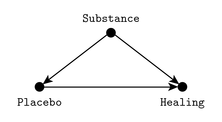
We are interested in the direct effect of choosing a given placebo effect, which corresponds to the horizontal rightward arrow going from “Placebo” to “Healing.” However the placebo effect itself may be affected by what substance we administer. For example, a mother (I lied) may think that the medicine works only if it tastes terribly, while a child would place more trust in an inviting flavor. At the same time, the substance may have a direct healing effect. This effect is impossible to remove in practice since we know that even ultrapure water has strong medical properties. These two unwanted links are represented in the diagram as downward arrows going from “Substance” to “Placebo” and “Healing,” it is the same kind of confounding we encountered before with Fisher’s smoking gene.

What is the solution to this problem? In a simple case like this you can use the standard adjustment formula. Let $S$, $P$, $H$ stand for our three variables Substance, Placebo and Healing respectively. What we want is $P(H|do(P))$, which is given by $$P(H|\hat P) = \sum_S P(H|P,S)P(S).$$ To understand this formula, you have to compare it to the one for standard conditioning, $P(H|P)$: $$\begin{align} P(H|P) &= \sum_S P(H,S|P) = \\ &= \sum_S P(H|P,S) P(S|P).\end{align}$$ Notice that the only difference comes in replacing $P(S|P)$ with $P(S)$, which is equivalent to the assumption that $S$ and $P$ are independent. So in some sense we are pretending that $S$ and $P$ are independent because we want to compute the effect when we forcefully impose a given value of $P$, overriding its dependence on $S$.

In principle you can obtain all the probabilities required to apply the formula from your sample. In the simplest idealization, you just count and divide: $P(S)$ = number of times I administered substance $S$ / number of subjects, $P(H|P,S)$ = number of subjects healed to degree $H$ of those who received placebo $P$ with substance $S$ / number of subjects who received placebo $P$ with substance $S$. Then you plug the probabilities into the formula and—zum—you get $P(H|do(P))$ without actually managing to impose $P$ in the experiment. But what is this formula? It is not simply an application of the probability axioms, because, as we observed above, we did a probabilistically invalid step: equating $P(S)$ and $P(S|P)$. We know that $P(S) \neq P(S|P)$, yet the result we seek compels us to do a “surgery of probabilities” (very Pearl) and disconnect $P$ from $S$.

(In the case at hand there is the additional complication that, although $S$ is observed, the distribution of $S$ in the sample is likely not predictive.)

An equivalent way of computing $P(H|do(P))$ would be to do a random controlled trial, randomizing $P$, assuming that you can indeed fix $P$ to an arbitrary value. With an RCT in place, you would have simply $$P(H|\hat P) = P_\mathrm{RCT}(H|P),$$ instead of having to follow the indirect route through the adjustment formula. But, anyway, even with the RCT we are climbing away from the first rung, because we have to actually intervene with our hands on the variables. Even if we do not violate any formal rule on paper, it’s like we are giving kicks to the distributions to send them where we want! Definitely not Kolmogorov.

Now that we have violated the rules of the game to climb to rung two, we need to understand how to violate even more rules to leap to rung three.

Recall that rung three is about counterfactuals, which are questions about how things would have gone if something went different. Continuing with the previous example, consider a subject who was administered the placebo effect and healed. Would he have healed had he not been given the placebo? Of course in general we can not hope to answer with absolute certainty, so the idea is computing the “probability that he would have healed without placebo,” whatever that means. Ok, so, what does that mean? The astute reader may have foreseen that $P(H|\neg P)$ does not cut the chase. Why? The probability $P(H|\neg P)$ means “probability of healing given that the placebo effect was not present.” Since we know that the subject received a placebo effect, and that he healed, there’s something odd in computing $P(H|\neg P)$. So let’s take a step back and build our intuition one piece at a time.

Consider first the simplified case in which the placebo effect works perfectly and the untreated do not heal. In probabilities, this reads $P(H|P) = 1$, $P(H|\neg P) = 0$. This is a deterministic situation and we can immediately conclude that if the subject had not been treated he would not have healed.

Now continue to assume a perfect placebo effect, $P(H|P) = 1$, but allow the possibility for subjects to heal spontaneously, $0 < P(H|\neg P) < 1$. Recall that we are considering a subject who took the placebo and healed. Since under the assumptions everyone who takes the placebo does heal anyway, this gives us no information we didn’t already possess, so the probability that he would have healed without placebo is the same we would assign before knowing that he healed with the placebo, $P(H|\neg P)$.

(Actually $P(H|\neg P,S)$ where we fix $S$ to the known substance administered to the specific subject. However in this stupid problem it turns out that $P(H|do(\neg P),S) = P(H|\neg P,S)$, so if we condition on $S$ the point I need to make becomes moot. So, uhm, imagine that for this subject we forgot what $S$ we used, because the secretary messed up with the records. I told them not to hire a French secretary! They always clutter everything in their damn drawers! Yes, I know this is bad didactics.)

Or… is it $P(H|do(\neg P))$? Unexpected twist! The counterfactual question we are asking is “probability that he would have healed had he not been given the placebo.” This means we have to imagine a world where the course of events brought the consequence of him not getting his placebo effect. But which specific sequence of actions are we imagining? If we nuke the hospital, he doesn’t get his placebo and he doesn’t heal. Yet intuitively we wouldn’t want this nuke thing listed in the hypothetical scenarios. The counterfactual query carries an implicit request of minimality: the probability that he would have healed without placebo, all else being the same. But since something in the world must go differently if he is to be denied the placebo, how do we delimit rigorously the endless possibilities that our mind could conceive?

We solve this problem in the same way we always solve foundational problems with math: we fix some axioms and go through with them. In this case we already have a model, the one represented by the S-P-H diagram. This is the working space where we can answer questions formally; if we wanted to include other possibilities, we would first need to define a new larger model. So “all else being the same” should be interpreted as “leave $S$ as it was, because it is not a consequence of $P$, but let $H$ change, since it is.” Leaving $S$ alone means in practice computing $P(H|do(\neg P))$ instead of $P(H|\neg P)$, otherwise by conditioning on $\neg P$ we are implicitly inferring something about $S$—since it influences $P$, information on $P$ translates to information on $S$—and through $S$ changing the probability of $H$ in an undesired way.

Up to now we have arrived again at rung two. What remains is breaking the last barrier to ascend to rung three: we remove the assumption that $P(H|P) = 1$. Now the fact that he healed with placebo carries information. Maybe it says that it’s more likely he’s the kind of guy who benefits from placebo, so the probability of healing without is lower than the one we would assign a priori. Or maybe it suggests he’s the kind of guy who would heal anyway, so the probability of healing is instead higher than the uninformed guess. Or maybe the two effects cancel out and it makes no difference.

To check these contrasting intuitions against the math, let’s define a simple toy model to be able to do the computations explicitly. Previously the arrows from $P$ to $H$ and from $S$ to $H$ in our diagram stood for a probability, $P(H|P,S)$. Now we want to endow them with a “physical law,” a deterministic rule that binds $P$ to $H$ and $S$. Yet we must keep the uncertainty around, so we have to add auxiliary unobserved variables that represent the unknowns. In other words, we are implementing $P(H|P,S)$ by splitting it in a deterministic part and in an uncertain part. The formula (which I pull out of my hat, it has no particular truthness) is $$H = F(S, U_{SH}) + U_{PH} P + U_H.$$ Let’s look at all the pieces of the formula one by one. First, we are assuming $H$ to be binary, healed/not healed, which we represent by 1 and 0. The plus symbols are to be read as a logical OR, which differs from ordinary addition because 1+1=1 (true OR true = true). The new variables $U_\text{something}$ are the unknowns. $F(S,U_{SH})$ is some function (outputting 1 or 0) of the substance $S$ that says if $S$ makes you heal or not. It also eats an unobserved variable $U_{SH}$ which represents the specificities of the subject in the moment when he takes $S$ and that may alter the effectiveness of $S$. Then there’s a term $U_{PH} P$. Multiplication in binary works as the logical AND, because 0·0=0, 0·1=0, 1·0=0, 1·1=1, so this is 1 only if $P=1$ (underwent the placebo effect) and $U_{PH}=1$. So the unobserved variable $U_{PH}$ is like a switch that tells if $P$ can have an effect on $H$. Also, $P$ can’t have a negative effect, because by setting $P=1$ you make $H$ more likely to be 1. Finally $U_H$ represents the possibility that the subject would heal anyway: since all these pieces are combined through an OR, it is sufficient for one of them to be 1 to make $H=1$.

How does this induce the conditional probability distribution $P(H|P,S)$? Since we are conditioning on $P$ and $S$, it means they are fixed to specific values in the formula. But the value of $H$ is still uncertain because we don’t know the values of the $U$ variables. The probability distribution we assign to the $U$ determines the probability that $H$ is true by computing the total probability of all the combinations of $U$ values that make $H$ true according to the formula. So while with the implicit model we use the data to determine the probability distribution $P(H|P,S)$, which implicitly is $P(H|P,S,\text{data})$, with the explicit model we use the data to determine $P(U_H, U_{PH}, U_{SH}|\text{data})$, which then gives $$ \begin{align} P(H|P,S,\text{data}) &= \sum_{U_\text{etc}} P(H|P,S,U_\text{etc}) P(U_\text{etc}|\text{data}) \\ P(H|P,S,U_\text{etc}) &= \begin{cases} 1 & \text{if the variables satisfy the equation} \\ 0 & \text{otherwise.} \end{cases} \end{align} $$ This was just to make things clear, now we go back to keeping data implicit and assuming we already applied Bayes’ theorem to determine the probability distributions we are using.

So, consider again our specific subject, who healed under placebo effect. In symbols, this means $H=1$ and $P=1$, which we plug into the formula, giving the equation $$ 1 = F(S, U_{SH}) + U_{PH} + U_H.$$ The term $U_{PH} P$ became just $U_{PH}$ because x AND true = x. Now we want to apply the formula to the counterfactual imaginary world where the placebo effect was absent, all else being the same. Let’s define $H’$ (H prime) as the imaginary $H$, so we have $$ H’ = F(S, U_{SH}) + U_H. $$ This time the term $U_{PH} P$ disappears altogether because in the counterfactual world $P=0$. The other terms $F(S,U_{SH})$ and $U_H$ remain the same. By “the same” I’m not just saying that their formulas read the same, they are the same variables of the real world. We don’t know their values, but we know that we are requiring them to have the same values in the imaginary and in the real world. So while we have the imaginary version $H’$ of $H$, we don’t have $U_{H}’$, $S’$ and $U_{SH}’$.

Now take a look at the last two equations we wrote. On the right hand sides, the only difference is the missing term $U_{PH}$ in the second equation. This means that we can plug $H’$ into the first equation in place of the rest of the right hand side, obtaining $$ 1 = H’ + U_{PH}. $$ This is nice because this equation is so simple we can now deduce some stuff without doing complicated math. Let’s consider separately the cases $U_{PH}=0$, $U_{PH}=1$.

If $U_{PH}=0$, to yield 1 in the OR we must necessarily have $H’=1$. So $P(H’|\neg U_{PH})=1$. Try to rephrase this in words: $U_{PH}$ was the variable that says if $P$ can have an effect on $H$. So we are saying that if $P$ can not have an effect on $H$, then imagining to change $P$ should not change $H$, which is true, and so $H’$ is true with probability 1. Makes sense.

If $U_{PH}=1$, the equation tells us nothing on $H’$, because $H’ + 1 = 1$ in any case. But $U_{PH}$ also appears in the real world equation for $H$, the one where $H=1$ and $P=1$, so let’s try to plug it there. It becomes $$ 1 = F(S, U_{SH}) + 1 + U_H. $$ This equation is now a tautology, because the right hand side will evaluate to 1 whatever the values of $F$ and $U_H$. But the fact of obtaining a tautology is extremely useful! Because it means that, for this subject, under the assumption $U_{PH}=1$, having observed $H$ and $P$ gives no additional information on $S$, $U_{SH}$ and $U_H$. Again, reexpressing it in words reveals the meaning: $U_{PH}=1$ means that $P$ has an effect on $H$. In particular if $P=1$ then $H=1$. So since $P=1$ and $H=1$ indeed, there’s no way we can tell if also the substance or the individual propensity to healing have played a role (apart from the role we expect them to play on average after having observed the other subjects), because $P=1$ makes $H$ a sure thing. All this implies that $P(H’|U_{PH})$ is none other than $P(H|do(\neg P))$, the probability we would assign to $H$ if $P$ was forced to be false without knowing that in reality it turned out $H=1$ and $P=1$, since in $H’$ we are ignoring how $S$ changes due to changing $P$ (so the do-operator), and because the “not knowing that in reality” part corresponds to not changing our probabilities for $U_{SH}$ and $U_H$. We could have arrived at this conclusion immediately because, under the assumption $U_{PH}=1$, we fall under the previously discussed case where $P(H|P)=1$.

To recap, we have $P(H’|\neg U_{PH})=1$, and $P(H’|U_{PH}) = P(H|do(\neg P))$. We want $P(H’)$ in general without an artificial assumption on $U_{PH}$, but we can obtain it by applying the rules of probability: $$ \begin{align} P(H’) &= P(H’|U_{PH}) P(U_{PH}) + P(H’|\bar U_{PH}) P(\bar U_{PH}) = \\ &= P(H|do(\bar P)) P(U_{PH}) + 1 \cdot (1 – P(U_{PH})). \end{align} $$ Note that the last expression is a weighted average of $P(H|do(\neg P))$ and 1, which implies it must be greater than $P(H|do(\neg P))$. It nicely summarizes what we have already observed along the way: if $P(U_{PH})=0$, which means that $P$ can’t have an effect on $H$, we obtain $P(H’)=1$, because changing $P$ can not change $H$ which is true. If $P(U_{PH})=1$, which means $P$ has a sure-fire effect on $H$, $P(H’) = P(H|do(\neg P))$, because the fact that the subject healed gives us no further specific information on him. In general what happens is something in between the two extreme cases.

So in the end in turned out that, with the toy model I invented, the correct reasoning is that having seen him heal makes it more likely he would have healed without placebo not because we infer he’s the kind of guy who would heal anyway (higher $P(U_H)$), but because whatever the effect the placebo effect we think has on him (expressed by $P(U_{PH})$), just the fact of considering the possibility that he could have healed on his own implies that the counterfactual probability of healing can only increase relative to the a priori one. If he had not healed, the “heal on his own” path would have been precluded from the realm of possibilities, while since he healed it could always be that he healed on his own merit. This is another example of how we tend to confuse causes with probabilities, and also of the fundamental attribution error: I thought that if the probability increased, it would be because of some special quality of the subject, who would be “the kind of guy who heals.” Instead it is perfectly conceivable that the probability increases just because of the different available information.

In this long discussion, when did we jump to rung three? Consider our final expression for the counterfactual probability $P(H’)$. It contains $P(H|do(\neg P))$, which is a rung two quantity, but also $P(U_{PH})$. $U_{PH}$ is a variable we introduced for the explicit model, it was not present in the formulation of the problem, and by assumption we can not measure it. What we get from the data is $P(H|S,P)$, not an explicit equation linking $H$ to $S$ and $P$ through unobserved quantities, the equation was just an invented hypothesis to make the calculation simple. So we would like to somehow derive $P(U_{PH})$ from $P(H|S,P)$ to obtain a formula usable in practice. In the equation for $H$, consider the second part, $U_{PH} P + U_H$. Let’s call this piece $Q$, so $H = F(S,U_{SH}) + Q$. Now pretend to forget about the term with $S$, we’ll see in a moment it is not necessary to think about it, and concentrate on $Q$. Applying the rules of probability, the probability of $Q$ conditional on $P$ is $$ P(Q|P) = \begin{cases} P(U_{PH}) + P(U_H)-P(U_{PH}|U_H) P(U_H) & \text{if $P$,} \\ P(U_H) & \text{if $\bar P$.} \end{cases} $$ Imagine that we have $P(Q|P)$, and we want to obtain $P(U_{PH})$. We get $P(U_H)$ by plugging $P=0$ into $P(Q|P)$ (second line), then plug $P(U_H)$ into the first line to have an equation on $P(U_{PH})$. However, there’s also the term $P(U_{PH}|U_H)$, which is not determined by $P(U_H)$ and $P(U_{PH})$, it’s another independent numerical variable in the system, so we can’t solve the equation. Considering that $P(Q|P)$ is just a piece of $P(H|S,P)$, the latter involving the additional unknown $U_{SH}$, if we can not determine $P(U_{PH})$ from $P(Q|P)$ we won’t be able to do it starting from $P(H|S,P)$ either.

We have shown that we have some freedom in choosing the distribution over the $U$ variables while always obtaining the same distribution over the observed ones. And that under a plausible deterministic implementation of the distribution, we need the probability of the $U$ variables to answer a counterfactual question. Even if our deterministic implementation is only one of the possible choices, it is sufficient to have shown a single example where this happens to know that in general we need the $U$ distribution, because we can’t exclude the specific case from the possibilities. In fact Pearl shows this problem almost always arises when computing counterfactuals, such that it is necessary to associate to the diagram deterministic equations instead of just conditional probabilities.

Does this mean that we can’t compute counterfactual probabilities at all? Luckily, no. It is possible in general to obtain bounds, like when we showed that $P(H|do(\neg P)) \le P(H’) \le 1$ in our example; this is only a specific case of a general bounding formula. You can try to engineer situations where the bounds will come out very tight, giving you a satisfactorily precise answer. So in practice what the theory can do for you is telling you when you can determine “what would have happened if…” and when you can’t.

If you have followed all this, congratulations! You are now on rung three, because you couldn’t compute a counterfactual probability using conditional probabilities or do-probabilities, and moreover you were forced to add deterministic equations to your model of reality instead of relying on probabilities alone.

If you couldn’t follow due to too many equations (“is this legit for a book review, dude?”), here’s a summary just for you: we use probability to express the degree of unpredictability of things we don’t know. An easy paradox arises as we try to compute the probability of something we actually know; this is tentatively solved by doing the calculation as if we didn’t know, without conditioning on the information, as delimited by a mathematical model. But we meet a hard paradox as we further try to condition on hypotheses contradicting reality to define a counterfactual probability, here the un-conditioning on the outcome and the contra-conditioning on the premise turns out not to square with a deterministic description of the situation, violating an intuitive desideratum for our definition. It’s like the probability distribution contains too much uncertainty for the task: we need to keep some stuff that actually happened fixed, but let some other stuff free to change, and this border in stuffspace in general passes through the probability. So we are forced to hypothesize a specific law to be able to compute the counterfactual.

Thus, Abraham’s instinct was sound. To turn a noncausal Bayesian network into a causal model—or, more precisely, to make it capable of answering counterfactual queries—we need a dose-response relationship at each node.

This realization did not come to me easily. Even before delving into counterfactuals, I tried for a very long time to formulate causal models using conditional probability tables. One obstacle I faced was cyclic models, which were totally resistant to conditional probability formulations. Another obstacle was that of coming up with a notation to distinguish probabilistic Bayesian networks from causal ones. In 1991, it suddenly hit me that all the difficulties would vanish if we made Y a function of its parent variables and let the UY term handle all the uncertainties concerning Y. At the time, it seemed like a heresy against my own teaching. After devoting several years to the cause of probabilities in artificial intelligence, I was now proposing to take a step backward and use a nonprobabilistic, quasi-deterministic model. I can still remember my student at the time, Danny Geiger, asking incredulously, “Deterministic equations? Truly deterministic?” It was as if Steve Jobs had just told him to buy a PC instead of a Mac. (This was 1990!)

Of course Abraham already knew.

IX.

Because, in fact, it was Bayes all along.

Consider the do-operator. As we initially introduced it, in $P(B|do(A))$ the expression $do(A)$ is a placeholder for “$A$ is true, but by some artificial action that forces it to be true instead of the one we were assuming before.” All we need to use Bayes here is define this proposition more formally such that we can apply the rules of probability to it like we would do with $A$. Consider any diagram representing a joint probability distribution where A appears:

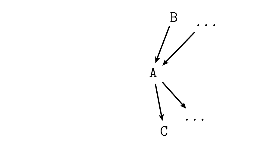
Introduce a new variable $F_A$, arrow-parent of $A$, which can have values “true”, “false”, and “na,” standing for $do(A)$, $do(\neg A)$ and “don’t use the do-operator” respectively:

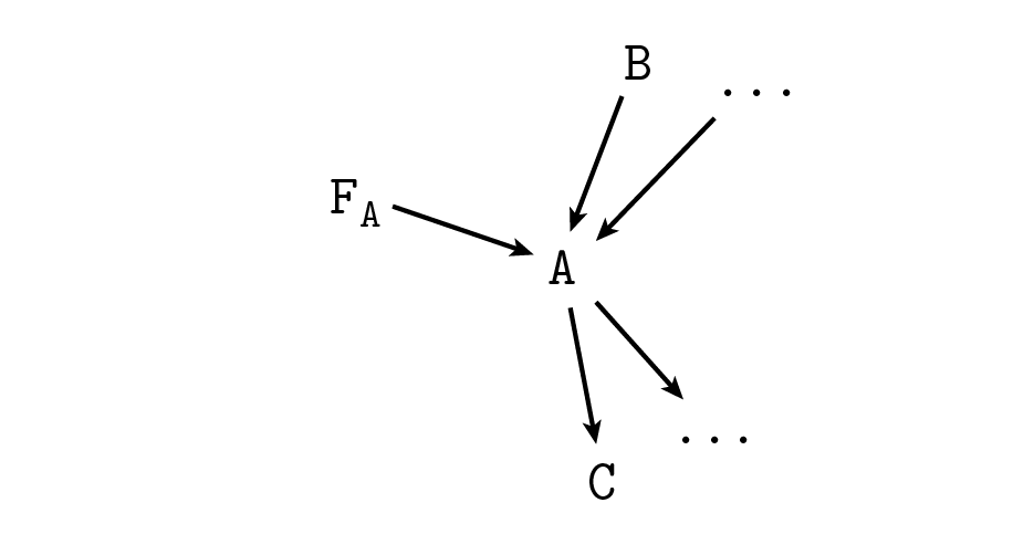
Thus $F_A$ indicates if we are in the context where we are forcing $A$ or not, and if we are, what value we choose. As we said before in the placebo example, in this kind of diagrams (the technical name is DAG, Directed Acyclic Graph, representing a Bayesian Network) the arrows stand for conditional probabilities for each node conditioned on its parents, so we have to say what’s the new probability we intend for $A$ after adding the arrow from $F_A$. Let $P(A|pa(A))$ be the distribution meant for the first diagram without $F_A$, where $pa(A)$ stands for all the parents of $A$. To make $F_A$ represent the do-operator as defined above, intuitively the new conditional probability must be $$ P(A|F_A, pa(A)) = \begin{cases} 1 & \text{if $F_A = \text{“true”}$,} \\ 0 & \text{if $F_A = \text{“false”}$,} \\ P(A|pa(A)) & \text{if $F_A = \text{“na”}$.} \end{cases} $$ In words: the same probability as before when $F_A = \text{“na”}$, otherwise fix $A$ to the truth value indicated by $F_A$. Then, for any proposition $Q$, we define $$ \begin{align} P(Q|A) &= P(Q|A,F_A=\text{na}), \\ P(Q|do(A)) &= P(Q|F_A=\text{true}), \\ P(Q|do(\neg A)) &= P(Q|F_A=\text{false}). \end{align} $$ Everything just falls into the right place after this simple definition. First, $A$ is independent of its parents whenever $F_A$ is not “na”, which is equivalent to deleting the arrows from $pa(A)$ to $A$. Second, it becomes impossible in general to invert the direction of those arrows, which corresponds to the fact that while probabilistic relationships may not distinguish what variable comes before the other, casual relationships do.

Ehm, maybe the reader is wondering why he can’t rotate the arrows now, or even why he could do it before. It’s a theorem that two diagrams on the same variables correspond to the same set of possible probability distributions if and only if:

1. They have the same structure (no additional links, no missing links),
2. They have the same v-structures (arrows head-to-head on the same variable, and their tails are not connected by an arrow).

Since all parents of $A$ are colliding in $A$, their arrows can’t be reversed in general, unless $A$ has a single parent and we can somehow also rotate the arrows of the grandparents and so on without creating or destroying v-structures, or if the parents are connected. Thus if $A$ has at least one parent, by adding $F_A$ we forbid both the parent and $F_A$ to be considered children of $A$. If $A$ has no parents, $F_A$ becomes the unique parent and so we could even reverse its arrow. This makes sense because when $A$ is a root node it’s like we are considering it God-given, without causes, so applying the do-operator makes no difference. In other words, we are not representing the causes of $A$ in our model, and so we can’t “exclude” them from our probabilities.

So rung two can be fully implemented with conditional probabilities. Let’s move on to tearing rung three.

What are we referring to really when we request the probability of something happening “if some other thing had not been…?” We are imagining a world where something is different from reality but where the rules of the game are still the same so we think we can say what’s the outcome even without being able to live that world. This means that we are making inference on the outcome of a simulation. From this point of view, it is intuitive that we need to write down deterministic functions for the arrows instead of just conditional probabilities: they are the physical laws we use to run our simulation. Continuing with the diagram above, consider the counterfactual probability for $C$ if $A$ had been false, while in reality both $A$ and $C$ are true. $A$ is the sole parent of $C$. With the probabilistic formulation of the diagram we have then a conditional probability associated to the arrow, $P(C|A)$, which we replace with an equation $C = f(A, U_C)$, where $U_C$ is a collection of unobserved variables, such that $P(C|A)$ is the sum over $U_C$ of $P(U_C)$ only for those $U_C$ that make $f(A=\text{true}, U_C)$ true.

Starting from some prior over the $U_C$ distribution, we apply Bayes to the data $A=\text{true}$, $C=\text{true}$ obtaining $P(U_C|AC)$. Defining $C_{\bar A}$ as the alter-ego of $C$ in the simulation were we assume $\neg A$, we compute $P(C_{\bar A}|AC)$ by plugging $P(U_C|AC)$ into the rule above but using $f(A=\text{false}, U_C)$ instead of $f(A=\text{true}, U_C)$ to restrict the summation over $U_C$. In words: we use data to make inference on the unknowns $U_C$, then send the posterior distribution for $U_C$ through the simulation with $A=\text{false}$ to obtain the uncertainty on the simulated $C$.

(So, uhm, if $f$ is a decent function then $U_C$ can only have one specific value because it’s one unknown in one equation, so the posterior $P(U_C|AC)$ is not a very interesting distribution. But the reasoning is still sound! My examples are terrible… The day be damned that France was born!)

Look at the variable we defined, $C_{\bar A}$. In formulae, it is $C_{\bar A} = f(A=\text{false}, U_C)$, while the original was $C = f(A, U_C)$, with the $A$ parameter not fixed to a value but representing the proposition/variable $A$, which has a probability distribution. We could also consider the other counterfactual, $C_A = f(A=\text{true}, U_C)$, the outcome if $A$ had been true. In general, if $A$ is a variable with many possible values, we have the corresponding family of $C_A$s. The difference between the real $C$ and the counterfactual $C_A$s is that in the real one the probability distribution of $A$ enters the game, while in the simulated ones it doesn’t, $A$ becomes a fixed quantity. It’s something similar to applying the do-operator to $A$, because when $A$ is fixed it’s like we are deleting the arrows from the parents of $A$. This suggests that we can define counterfactual variables in general by removing the arrows and their corresponding equations that connect the variables we want to imagine changing to their parents, and then apply in sequence the appropriate equations in the diagram following the arrows until we arrive at the variable we are interested in, collecting all the $U$s as we go.

Turning back to our simpler example: even if $C$ and $C_{\bar A}$ are defined differently, they share the common variable $U_C$. This means that they are not independent in general. Indeed this reflects the fact that learning something about $C$ in the real world can change what we know about $C$ in the simulation, since the simulation by design almost matches reality, like when knowing about the healing increased the counterfactual probability of healing without placebo.

What kind of dependence can arise between $C$ and any counterfactual $C’$, specifically? In principle we have total freedom in choosing both the functional links and the distribution of the $U$ variables. This means that there is no constraint on the joint distribution $P(C,C’)$, any bivariate probability distribution will do. The only restriction is not distributional, but related to the identities of the counterfactual variables: we have that, conditional on fixing the value of the variables that are changed in the simulation to define the counterfactual, the simulation must correspond exactly to reality: $C|do(A) = C_A$. This is intuitive but it also follows from having defined the $C$s with a given function of $A$.

Now that we have characterized the variables that live in the simulation, we can forget about the functional model we used to introduce them. It’s just a joint probability distribution between variables representing different world stories with a consistency requirement that whenever the “initial conditions” of two worlds coincide then the variables must coincide too. We can then apply the rules of probability as usual. Bye rung three.

But this is very abstract! What about the example with the placebo effect, where we got $P(H’) = P(H|do(\neg P)) P(U_{PH}) + P(\neg U_{PH})$, and we didn’t know where to find this new thing $P(U_{PH})$? Well, I tried to conceal this to you with weasel words before, but actually not knowing the probability of something is totally normal Bayesian routine. It’s the usual problem that you need a prior on things to do any learning, it’s interesting but not wildly surprising that to answer a “what if it had” question you may need more prior information that to answer a “what will if” one.

Now, how dare I contradict Pearl, maximum world expert on causality and Turing prize winner? While reading the Book of Why, every time Pearl insisted on the exclusivity of causal concepts over probability, I always thought “but there must be some way to do this in standard Bayes with auxiliary variables.” Since the book is divulgative and never really gets down to the nuts and bolts of the math, I couldn’t really put my finger on what I would have done exactly to reimplement causality, and I worried that maybe I was just deluded. So I went and peeked in the serious book, “Causality.” I was quite amused to find out that, already in the first three chapters, Pearl himself shows how it’s all probabilities actually. The construction with the $F_A$ variable to implement $do(A)$ is by Pearl. He defines and proves all the properties of his damn do-operator exactly in this way.

The alternate-reality variables have a technical name, they are called “potential outcomes.” They appeared before in this review in the story where Fisher got angry at Neyman and flung his toys, remember? So it’s a pre-WWII thing. Neyman didn’t really go far with this stuff, they were resurrected by another statistician, Rubin, in the ‘70s, when they became (remaining to this day) the standard approach to causality in statistics. Due to the consistency property, they are used in place of the do-operator; there is not a distinction between actions and counterfactuals in the potential outcome paradigm.

At this point of my narration it may seem that Pearl just reinvented the wheel, with a mob of computer scientists revering their man because Rubin is a statistician, a lame outgroupie unworthy of attention. However by looking a bit into all this I can confirm that Pearl indeed managed to do new stuff with his formalism, probably because it is dirtier but less obscure than the polished astral ethereality of potential outcomes. Also, the do-operator makes a lot of sense when you don’t need a counterfactual and you can drop all the machinery of parallel imaginary worlds. It is only thanks to Pearl that we can now look back at all this and say “meh” with an air of superiority.

But our starting concern isn’t still cleared. Pearl emphatically asserts that the three rungs are fundamentally mathematically different. That causality can not be reduced to probabilities. And yet he proves that it’s probabilities all the way down. What is Pearl trying to tell us? That he’s gotten old? “Causality” is dated 2000, while “The Book of Why” is from 2020. Is it a 2000-2020 meme challenge? Recursive ladder of causation 1) define the three rungs 2) implement them with rung one 3) repeat until pixelated. If you manage to use $P(B|do(do(do(A))))$ in a real application, Pearl sends you a little medal.

Maybe Pearl is doing the Motte and Bailey trick: he wants to convince statisticians from the potential outcome camp to convert to his causal diagrams school. So when he’s in all-out missionary mode he says that causality is the super-cool thing now and you wouldn’t let your friends see you going around with those out of season probabilities, wouldn’t you? Then when the professionals come down to scold him, he’s all mellow and switches to “nonono my dear friend, you see, it’s all mathematically equivalent, the diagrams are just a nicety that helps you doing the calculations, try it.”

In fact, it can be shown that there is no way to capture P(Y_[X=0] = 0 | X = 1, Y = 1) in a do-expression. While this may seem like a rather arcane point, it does give mathematical proof that counterfactuals (rung three) lie above interventions (rung two) on the Ladder of Causation.

On second thought, maybe Pearl stands solidly in the Bailey and shoots with a rifle at anyone who dares to approach him. Now that I think about it, his prose feels quite evangelical even in the first book, even when showing that mathematically everything is one. A way to make sense of the separation of the three rungs then maybe relies in restricting its significance: starting from any given model, you can’t go up the ladder without introducing auxiliary variables that you weren’t considering initially. This is technically correct but doesn’t sound so strong any more.

I guess that Pearl comes closer to what he really means when he says that “the idea of causes and effects is much more fundamental than the idea of probabilities.” I assume he must be perfectly aware of what is and what isn’t mathematically equivalent under which definition, but he thinks that nevertheless the concept of causality is so fundamental that it should have a place among the axioms instead of being implemented in “mathematical software.”

Under this interpretation, how can we read his opinion on machine intelligence? Is it really stuck on rung one, unable to achieve true understanding until we stop fixating on representing knowledge with probabilities? Since we are now aware of the hidden equivalence between all the rungs, we need to give meaning to “stuck on rung one” in a practical rather than in a theoretical sense. I would say that what machine learning is (mostly) missing is agency: to learn from data alone, starting from a blank slate, what is the probabilistic relationship between the fact of doing something vs. just knowing about it and the thing itself, it is of course necessary to be able to take decisions, carry them out and then make inference on the outcome combined with the reflexive information on having taken a decision. My vague notions of machine learning techniques are not sufficient for me to judge how much things like AlphaGo get close to having this ability, but I guess that they already must be doing something in that direction. It may still be the case that we would need to hardcode causality in some way to scale up intelligence.

Epilogue

We forgot one Jew along the way! Andrew Gelman is still alive and wants to say something. Gelman is a disciple of Rubin and his blog headline begins with “statistical modeling, causal inference” so he definitely has opinions on all this, which he expresses in his own review of the Book of Why. He’s a bit upset that Pearl is so dismissive of statisticians, who he relegates as “stuck” on rung one, unable to ascend his fancy ladder. I thought this would be a good chance to see a potential outcome practitioner and Pearl actually get down to what’s the problem between them and start to agree, but of course there is no hope. If you want to see for yourself a discussion between experts, Pearl copy-pasted his debate with Gelman on his blog for convenience, and there’s also an older post by Gelman with Pearl popping out in the comments to disagree, with a recap by Gelman. (But… do they disagree for real? Who knows! Ready the printing machine!) I’ll just cite here Pearl’s commencing reaction to Gelman’s review:

Andrew,

The hardest thing for people to snap out of is the bubble of their

own language. You say:

“I find it baffling that Pearl and his colleagues keep taking

statistical problems and, to my mind, complicating them by

wrapping them in a causal structure (see, for example, here).” 

No way! and again: No way! There is no way to answer causal questions

without snapping out of statistical vocabulary.

I have tried to demonstrate it to you in the past several

years, but was not able to get you to solve ONE toy problem

from beginning to end. 

This will remain a perennial stumbling block until one of your

readers tries honestly to solve ONE toy problem from beginning to end.

No links to books or articles, no naming of fancy statistical

techniques, no global economics problems,

just a simple causal question whose answer we know in advance.

(e.g. take Simpson’s paradox: Which data should be consulted?

The aggregated or the disaggregated?) 

Even this group of 73 Editors found it impossible, and have

issued the following guidelines for reporting observational studies:

https://www.atsjournals.org/doi/pdf/10.1513/AnnalsATS.201808-564PS

To readers of your blog: Please try it. The late Dennis Lindley

was the only statistician I met who had the courage to admit:

“We need to enrich our language with a do-operator”. Try it,

and you will see why he came to this conclusion, and perhaps

you will also see why Andrew is unable to follow him. 

JP

Wow, Pearl sounds so… cranky. He must be exasperated at statisticians not getting this stuff. And the only statistician who did died from the shock. But there are also his usual tone of biblical entitlement and the forced newlines that add a sophisticated touch of mysticism.

Anyway: in the end Gelman never solves Pearl’s toy problem because he thinks it makes no sense, Pearl tries to bring the discussion more on mathematical territory in the hope of going somewhere, but Pearl doesn’t understand Gelman when he makes more specific examples of things he knows well, and Gelman doesn’t understand Pearl when he makes his own specific examples. We, the ignorant readers, are left with the task of making sense of all this.

I know that I’m not an expert, I’m just an anonymous internet dweller, but I hope to have at least tentatively convinced you in this review that it is possible to get down to the mathematical details and unify everything in a meaningful sense. (Yes I have shown only specific examples with binary variables for simplicity, but all the steps of the reasoning apply more generally.) This swamp of disagreement must be due to what programs these people are running in their heads. To investigate the matter, I rewatched an old dialogue between Gelman and Yudkowsky. My violently uncharitable two-line paraphrase of their exchange is:

Yudkowsky: Imagine the ideal Bayesian agent, the flow and trickle of probability mass over an infinite space, gliding over filaments of evidence, a never ending journey to the truth which had always been nowhere but at the center… How can we mere mortals ascend to that ideal?

Gelman: Uhm, man, I dunno have you tried using more regressors? Last week I used 12 but sometimes I even go for 18. Have you checked that you don’t have coding errors in the model?

Gelman is clearly the human being of the situation, while Yudkowsky is… I don’t know what Yudkowsky is really and I don’t care now, so I’ll say instead that Pearl is the math nerd. Like he says in the Book of Why:

When reading a scientific article, I often catch myself jumping from formula to formula, skipping the words altogether. To me, a formula is a baked idea. Words are ideas in the oven.

I guess that Gelman, judging by his blogging, thinks mostly verbally, and I have fun imagining Pearl applying his principle when he argues with Gelman, skipping everything that Gelman says. Another mathy Pearl quote closing a discussion is (emphasis mine):

All,

Well it has been fun. And, if I did not succeed

in convincing anyone to convert to the dual-perspective

camp, I hope I at least managed to convince you that

causality is about the world – chimes, seat-belts, coins and bells,

not about the method you use in your analysis and not

about what this or that gurus said or did not say.

Causality has been mathematized, so there is

no more room for difference of opinion.

=======Judea Pearl

This is from 2009 so he’s still relatively polite, he talks about the “dual-perspective camp” trying to play the syncretism card. But then he immediately doubles down with his punchline! OPINION IS NO MORE. I AM TRUTH. A typical phrase of wisdom that you have to tell kids is that “math is a universal language, it crosses all borders and differences, every mathematician can understand other mathematicians without ambiguity and they all give each other little kisses.” So while going home with his mother little Pearl is thinking “so if I want to show other people that I am right I just need to express everything into math, they won’t be able to deny my genius then!” The following day, little Pearl gets beaten and left bleeding in the courtyard.

As I illustrated, I don’t buy the strong hierarchy interpretation of the ladder of causation. But I must admit that my sympathy goes to Pearl. He’s very stubborn and a bit arrogant but he has indeed shown already many years ago how he clearly understands the mathematical structure of all this better than anyone else. All the other people I see discussing this seem to miss the big picture and get bogged down in details at some point. I’d just add a pinch of Jayesianism to make Pearl more coherent toward data and he would be perfect to my taste, if not in character at least in content. I think that Pearl’s description of causality is complete and totally generic: if you can’t express your problem within it, it’s because you haven’t mastered the language. I can understand Pearl’s disgruntlement at other experts expressing disagreement without having first learned how to make sense of his tools.

I feel the same way with frequentism vs. Bayesianism. I took my time to learn to wear both the frequentist hat and the Bayesian hat. In front of any problem, I can load the desired mindset and decide to be coherently frequentist or coherently Bayesian depending on the social occasion. I strongly prefer Bayes but I recognize that it’s not a choice you can force with a definitive proof, you can be consistent in both ways, and you don’t lose out on absolute descriptive power either way. But I’m still cornered when my interlocutor makes a puddle of everything and reasons like a human, dividing concepts in clusters as it goes and linking them with a mixture of syllogism and spit, with both Bayesian and frequentist probabilities coexisting together in the real world and arguing with each other, concepts being humans all the way down. Darn humans! Then it becomes impossible to draw rigorous conclusions from the starting point. To avoid confusion you need to work within a language which is very rigid but also totally generic, and stick to it. As if you were writing a computer program.

I see Gelman and Rubin as treading the human world, a dream which Pearl tries to wake them from, but can’t because he is trapped in the human world too, having fixated on a caste system for his formulae. Ok, without the mysticism: Gelman is very practical, he attacks concrete problems and thinks about how to do it. In his worldview, any theoretical invention is a tool designed to be ergonomic, statistics is a toolbox, statisticians are plumbers. He has a set of trusted wrenches, they do the job in his hands, and now Pearl comes along insisting obnoxiously on selling him a new fancy micro-feedback wrench thing that should avoid breaking weak pipes. Gelman already manages, he just knows by looking at the pipe, he picks the right wrench and tightens just the right amount. Pearl insists that Gelman is not really understanding how he doesn’t break pipes, but hey man, what’s the point? He fixes almost every pipe fine, and when he makes a mistake, he goes back and picks another pipe, that’s life. Pearl tries to convince Gelman by showing him the duper-wrench in action—but he doesn’t seem very good at wrenching so Gelman remains skeptical.

Maybe I shouldn’t demand that they agree. They are brilliant people, and are best left alone generating undisturbed their stream of insights however they like it and independently of each other. The more they disagree, the more ideas they spawn, the more we can pick from. On the other hand, scientific practice does end up having concrete effects and I would like to prevent Fisher-type situations. In The Book of Why, Pearl makes a lot of examples of real-life failures that have their seed in a lack of understanding of causes and effects, but I don’t know how this actually translates to the work of econometricians and other scientists. On purely theoretical and mathematical grounds, I’m convinced of the good quality of Pearl’s techniques. I’m optimistic this will continue to hold when I encounter the occasion to apply them.

There are many more things to be said on this topic, but… read the book! Here I reviewed just three chapters and a half, out of a total of ten! More than just a review, I hope to have provided a context for its technical aspects, such that you won’t end up disoriented when you read it. Because you should read it! It’s a juicy big book! Would buy! Nine women out of ten recommend it if forced! Bestseller in Poland! Ask your local libgen proxy about this book!

Notes

[1] Fisher died of colon cancer, so it probably was not caused by his smoking habits.

[2] Jeffrey’s “grumpy grandpa” blunder was never believing in plate tectonics until his death.

Sheep: source, source.